Lab 7: Hypothesis Testing - Paired Groups

Digital Accessibility

Please note that all images were created with modifications to the defaults to make them digitally accessible. If you recreate this code in another environment, your plots have different colors and backgrounds.

1 Getting Started

Be sure to load the packages ggformula and mosaic, using the library() function. Remember, you need to do this with each new Quarto document or R Session. Add the package names in each of the blanks below to load in the indicated packages.

library() loads in packages. You need to supply the package name you need to load inside the parentheses.

library(ggformula) #for graphs library(mosaic) #for statistics library(tidyverse) #for data management

library(ggformula) #for graphs
library(mosaic) #for statistics
library(tidyverse) #for data management

Revisit Lab 5 Primer

The examples used in the Lab 6 Primer are continuations from the Lab 5 Primer. We encourage you to go back and review your previous answers and code to help you with your lab.

2 Birth Parents Age Gap

A recent study found the average Homo sapiens father has always been older than the average Homo sapiens mother for 250,000 years. However, the age gap has dwindled in the last 5,000 years, largely due to mothers having children at older ages. With declining teen birth rate, rising birth rates among older women, and women pursuing higher education and careers before starting families, the average age of all mothers giving birth in the United States increased to nearly 30 in 2023. While the age gap between parents can vary greatly, it’s common for fathers to be just a few years older than mothers.

The National Vital Statistics System (NVSS) is a collaborative effort between state and local governments in the US to compile and publish reports on all vital events - births, deaths, marriages, and divorces. A random sample of 50 births in 2022 was extracted from NVSS. The data for mother’s age and father’s age can be found in nvss-births-2022.csv.

The researchers want to determine if the age gap still exists and if fathers are still older than mothers.

Run the following code chunk to read in the data and view the variable names.

2.1 Identify the Parameters

Identify the study design of this study.

Be sure you are able to provide a full justification. This is review from the Lab 5 Primer.

Independent Two Sample
Matched Pair Sample

Identify the correct parameter type for this study. Be sure you are able to complete the full parameter in context.

True mean difference
Difference in true means

Identify the parameter(s) that would be of interest based on the study design.

μₓₓ = true mean age in years of mothers
μₓᵧ = true mean age in years of fathers
μₓᵧ₋ₓₓ = true mean of the differences of the ages in years of fathers and mothers
x̄ₓₓ = mean age in years of mothers in our sample
x̄ₓᵧ = mean age in years of fathers in our sample
x̄ₓᵧ₋ₓₓ = mean of the differences of the ages in years of fathers and mothers in our sample

Identify the null hypothesis that would be of interest based on the study design.

The researchers want to determine if the fathers’ ages are greater than the mothers’ ages at birth.

μₓᵧ - μₓₓ = 0
μₓᵧ - μₓₓ < 0
μₓᵧ - μₓₓ > 0
μₓᵧ - μₓₓ ≠ 0
μₓᵧ₋ₓₓ = 0
μₓᵧ₋ₓₓ < 0
μₓᵧ₋ₓₓ > 0
μₓᵧ₋ₓₓ ≠ 0

Identify the alternative hypothesis that would be of interest based on the study design.

The researchers want to determine if the fathers’ ages are greater than the mothers’ ages at birth.

μₓᵧ - μₓₓ = 0
μₓᵧ - μₓₓ < 0
μₓᵧ - μₓₓ > 0
μₓᵧ - μₓₓ ≠ 0
μₓᵧ₋ₓₓ = 0
μₓᵧ₋ₓₓ < 0
μₓᵧ₋ₓₓ > 0
μₓᵧ₋ₓₓ ≠ 0

2.2 Exploratory Data Analysis

Recall from the Lab 5 Primer, we calculated the following summary statistics and data visualizations.

2.2.1 Summary Statistics

df_stats(~(FatherAge - MotherAge), data = parents) 

                  response min Q1 median Q3 max mean       sd  n missing
1 I(FatherAge - MotherAge) -13  0      1  4  17  1.8 4.952839 50       0

2.2.2 Data Visualization

gf_boxplot(~(FatherAge - MotherAge), data = parents,
           xlab = "Difference in Ages Between Fathers and Mothers") |> 
  gf_theme(axis.ticks.y = element_blank(),  #removes y-axis ticks
           axis.text.y = element_blank())   #removes y-axis labels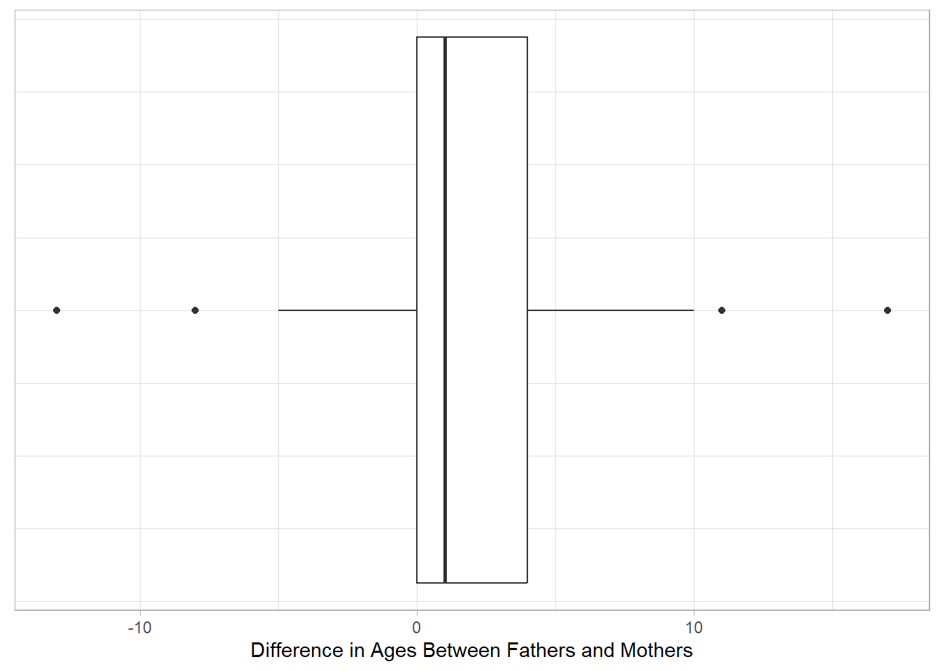

2.2.3 QQ Plot

gf_qq(~(FatherAge - MotherAge), data = parents,
      ylab = "Difference in Ages Between Fathers and Mothers",
      xlab = "Theoretical Z-Scores") |> 
  gf_qqline()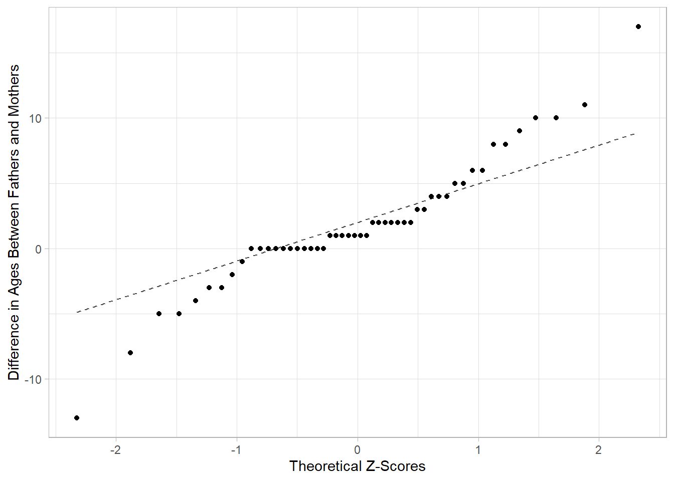

Based on the provided information, do we meet the necessary conditions to conduct inference using the t-distribution (e.g. confidence interval, hypothesis test)?

Yes, because we have random sample
Yes, because our sample size is greater than 30
No, because our sample data is skewed

• Remember to check the conditions of sufficient sample size and normality together.
  
• The sufficient sample size depends on whether our sample indicates the population may or may not be normality distributed (now evaluated using the QQ Plot).
  
• Provide a statement, based on the condition check, to determine if we can or cannot use the t-distribution as a model for null distribution or sampling distribution of our test/sample statistic.

2.3 Calculating the Test Statistic and P-Value

We will practice code for both a “by-hand” calculation and using t.test() (which is what we will be using from in general).

Calculate the summary statistics for each sample. Modify the code below to calculate the summary statistics for each group.

You should get the following values:

mean_diff	sd_diff	n_diff	effect_diff
1.8	4.952839	50	0.3634279

2.4 Calculating a t-Test Statistic and p-Value for the Mean of the Differences

Now that we have the necessary summary statistics saved, we can calculate both our test statistic (t) and our p-value. Recall the t-statistic for an matched pairs test is

\[t_0 = \frac{\bar{x}_{d} - d_0}{\frac{s_{d}}{\sqrt{n_{d}}}}\]

Fill in the blanks below using the saved object names (e.g. mean_diff, sd_diff) from above.

Now, calculate the p-value using the pt() function. Consider the direction of the alternative hypothesis.

1-pt(t, df = n_diff - 1)

1-pt(t, df = n_diff - 1)

Test statistic: Round to 4 decimal places.

df:

p-value: Round to 6 decimal places.

Now, let’s calculate the test statistic and p-value using the t.test() function. Consider the direction of the alternative hypothesis. Recall you have three choices for the alternative.

• "two.sided"
  
• "greater"
  
• "less"

t.test(~(FatherAge - MotherAge), data = parents, mu = 0, alternative = "greater")

t.test(~(FatherAge - MotherAge), data = parents, mu = 0, alternative = "greater")

2.4.1 Switching the Direction of the Difference

Ultimately, it is up to the researcher to choose the direction of the calculated difference. If we wanted to switch our difference and have Mother’s Age - Father’s Age we would have to tell R to change the ordering of inside each of our functions.

Rerun the t.test() code, but calcuate the differences between Mother’s Age and Father’s Age instead of the other way around. What do you have to change to make the test equivalent?

t.test(~(MotherAge - FatherAge), data = parents, mu = 0, alternative = "less")

t.test(~(MotherAge - FatherAge), data = parents, mu = 0, alternative = "less")

2.5 Interpreting and Evaluating the p-Value

Using the calculate p-value from the t.test() function to answer the following questions. (Use the original ordering of Father’s Age - Mother’s Age).

Which of the following are correct interpretations of a p-value?

The probability of observing our test statistic
The probability of observing our test statistic or greater
The probability of observing our test statistic or greater, assuming the null hypothesis is true
The probability of observing our test statistic or greater, assuming the alternative hypothesis is true
The probability that the null hypothesis is true
The probability that the alternative hypothesis is true
The probability that we find evidence against the null hypothesis

Evaluate the strength of evidence against the null hypothesis, using a significance level of \(\alpha = 0.05\)

no evidence
little evidence
some evidence
moderate evidence
strong evidence
very strong evidence

Full Evaluation of Strength of Evidence

Remember we have specific details to include in a full evaluation of the strength of evidence.

We have {very strong/strong/moderate/some/little} evidence against the null hypothesis (in favor of the alternative hypothesis) that {context of indicated hypothesis} (t = {xxx}, df = {xxx}, p-value = {xxx}).

Which of the following statements are true based on the p-value?

there is a very small probability the null is true
our data/test statistic is very unlikely to be observed if the null is true
there is a very small probability the alternative is true
there is a very large probability the alternative is true
there is a very small probability of finding evidence against the null

Which of the following are possible, given the results of the hypothesis test?

Our result is a Type I Error
Our result is a Type II Error
Our result is Correct

Which is the best definintion of Power in the context of the study?

The probability of finding no evidence of a difference in the age of parents, when there is a difference
The probability of finding no evidence of a difference in the age of parents, when there is no difference
The probability of finding evidence of a difference in the age of parents, when there is a difference
The probability of finding evidence of a difference in the age of parents, when there is no difference

2.6 Calculating a Confidence Interval for the Mean of the Differences

In order to calculate the confidence interval for the population mean of the differences, it takes on the same structure as a confidence interval for one population mean.

\[point \ estimate \pm (critical \ value)*(standard\ error)\]

or

\[\bar{x}_d \ \pm \ t^*\frac{s_d}{\sqrt{n_d}}\]

We can find our \(t^*\) critical value the same way we found it for previous confidence intervals.

Our point estimate is \(\bar{x}_d\)

and finally we can calculate the lower bound (lb) and upper bound (ub) for our confidence interval.

Record the calculated confidence interval.

Lower bound:

Upper bound:

Of course, the “by-hand” method is tedious when we can just use t.test() to calculate our confidence interval. Fill in the blanks below to calculate the 95% confidence interval for the difference between the two means.

t.test(~(FatherAge - MotherAge), data = parents, conf.level = 0.95)$conf.int

t.test(~(FatherAge - MotherAge), data = parents, conf.level = 0.95)$conf.int

Provide an interpretation of the confidence interval by reordering the phrases below.

of the differences between

the age of mothers

the age of fathers

LB and UB

and

the true mean

we are 95% confident that

Based on the sample

is a single value

within the interval

Which of the following would be plausible estimates for the true mean of the differences between fathers’ and mothers’ ages?

0
-1
1
-1.5
-0.5
0.5
1.5
-2
2

What can we conclude about the study?

we cannot infer that the age of the mother causes the age of the father to be higher
we can infer that the age of the mother causes the age of the father to be higher
there is evidence that fathers tend to be older than mothers in 2022
there is no that fathers tend to be older than mothers in 2022
the effect size indicates a large difference between the ages of fathers and mothers
the effect size does not indicate a large difference between the ages of fathers and mothers

Indentify the population to which you can generalize.

all Homo sapiens
all birth parents
all US birth parents
all US birth parents in 2022
all parents with an age gap
none